[Perceptron] Single and Multi-Layer Perceptron

1. Neuron

The idea of perceptron stems from the human’s neural network system. A ‘Neuron’ is one unit that consists of the whole neural system. In 1943, Doctor Warren McCulloch and Walter Pitts had suggested a concept of artificial computerised neuron, which is a ‘Perceptron’.

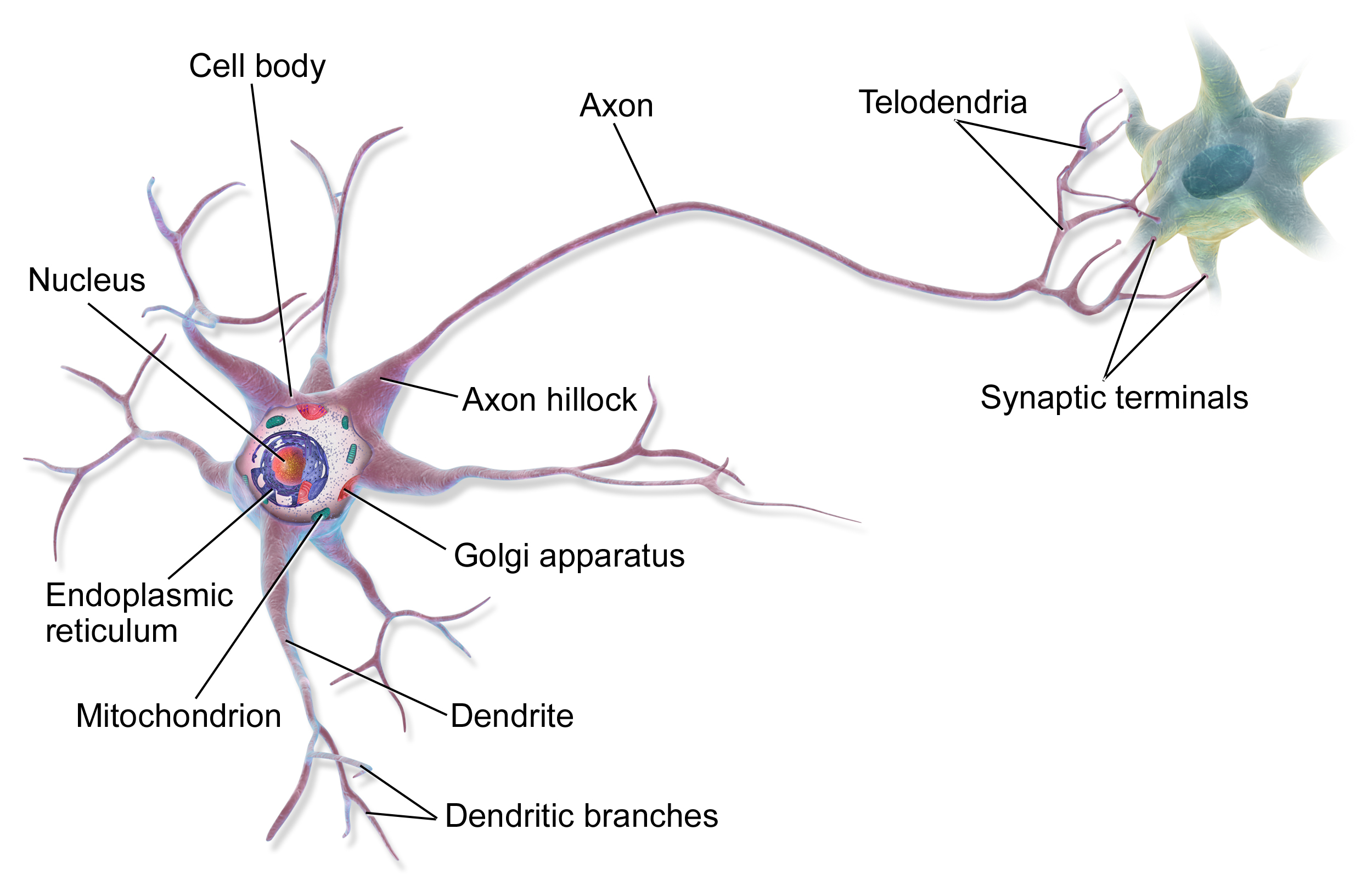
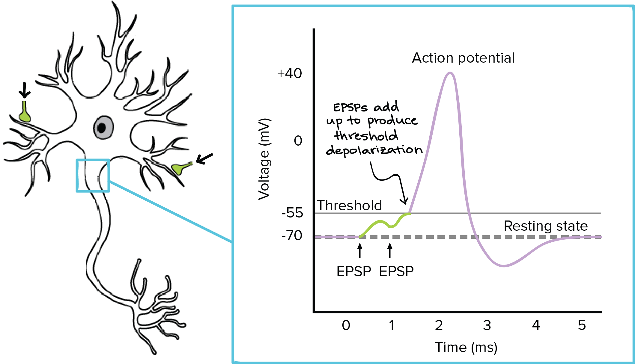
The image above is a descriptive drawing of a biological neuron. Neurons are connected in a really complex order with each other, and an output signal from one neuron cell heads to the dendrites of its adjacent neuron cell, acting as an input signal to that neuron cell. Those input signals are accumulated in a cell body, and if the accumulated signals exceed a certain threshold, an output signal travels out from the cell through Axon and Telodendria. Below is an image from Khan academy synapse explanation, which can help you understand the concept of threshold.

2. Single Layer Perceptron

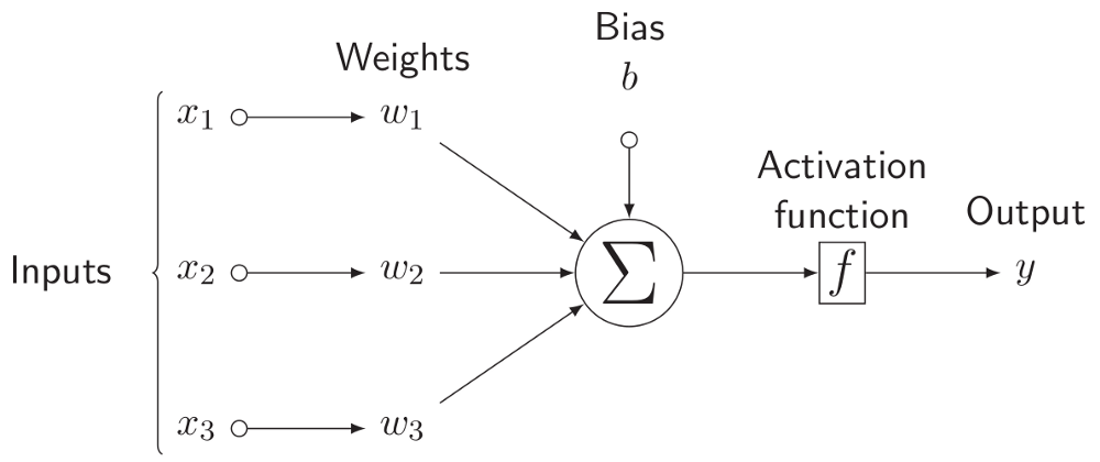Similar to the biological neuron, perceptron has an activation function that decides whether it should output the value or not - as 0. (You will know this is not actually a precise sentence in section 4, but for now, you can understand activation function like i mentioned.)
Therefore, an activation_function would be as below.

def activation_function(y):
    if y <= 0:
        return 0
    else:
        return 1

2-1. Implementing Logic Gates with perceptrons

By using the activation_function above, we are going to implement some famous logic gates with perceptron.

1. AND Gate

   def AND_gate(x1, x2):
    x = np.array([x1, x2])
   
    # these are the weights that are to be multiplied by x1 and x2
    w = np.array([0.5, 0.5])
   
    # bias
    b = -1 * w[0]
   
    # perceptron
    y = np.sum(w * x) + b
   
    return activation_function(y)
   

2. OR Gate

   def OR_gate(x1, x2):
    x = np.array([x1, x2])
    w = np.array([0.5, 0.5])
    b = -0.2
    y = np.sum(w * x) + b
   
    return activation_function(y)
   

3. NAND Gate

   def NAND_gate(x1, x2):
    x = np.array([x1, x2])
    w = np.array([-0.5, -0.5])
    b = 0.7
    y = np.sum(w * x) + b
   
    return activation_function(y)
   

print('OR Gate')
for x1, x2 in array:
    print('Input: ', x1, x2, ', Output: ', OR_gate(x1, x2))

print('NAND Gate')
for x1, x2 in array:
    print('Input: ', x1, x2, ', Output: ', NAND_gate(x1, x2))

print('AND Gate')
for x1, x2 in array:
    print('Input: ', x1, x2, ', Output: ', AND_gate(x1, x2))

# Terminal output
# OR Gate
# Input:  0 0 , Output:  0
# Input:  0 1 , Output:  1
# Input:  1 0 , Output:  1
# Input:  1 1 , Output:  1
# NAND Gate
# Input:  0 0 , Output:  1
# Input:  0 1 , Output:  1
# Input:  1 0 , Output:  1
# Input:  1 1 , Output:  0
# AND Gate
# Input:  0 0 , Output:  0
# Input:  0 1 , Output:  0
# Input:  1 0 , Output:  0
# Input:  1 1 , Output:  1

3. Multiple Layer Perceptron

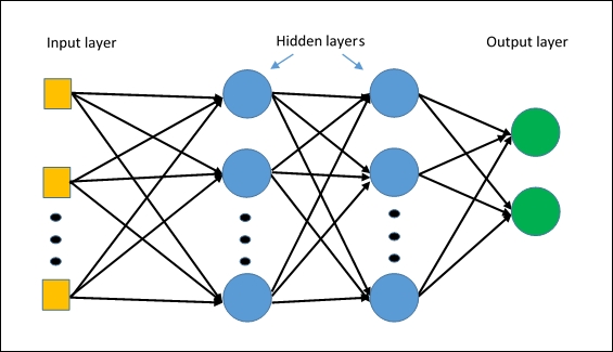
By connecting multiple number of single perceptrons like our body does, you can create much more complex and efficient structure and we call that Multi Layer Perceptron (MLP). Because it has multiple layers, there is a presence of at least one hidden layer, which is not actually connected to the inputs and outputs of the structure. MLP will be discussed much in detail from the next blog post, which is about training the network.

3-1. Implementing XOR Gate with multiple perceptrons

With Multiple layers of perceptron you can implement one more logic gate that you couldn’t do with just single perceptron. It is XOR Gate.

1. XOR Gate

   def XOR_gate(x1, x2):
    NANDed = NAND_gate(x1, x2)
    ORed = OR_gate(x1, x2)
    return AND_gate(NANDed, ORed)
   

4. Activation Functions

Let’s find out some more activation functions.
But before we go on, keep in mind how np.maximum() function works!

print(np.maximum(0, np.array([0.5, 0.4, -0.2])))
# this is the output: [0.5 0.4 0. ]

4-1. Type of activation functions

• Softmax activation

\[softmax(x_{i}) = { e^{x_i} \over \sum_{j}e^{x_j} }\]

def softmax(x):
    nominator = np.exp(x)
    denominator = sum(np.exp(x))
    return nominator / denominator

• Sigmoid activation

\[sigmoid(x) = { 1 \over 1 + e^{-x} }\]

def sigmoid(x):
    denominator = 1 + np.exp(-x)
    return 1 / denominator

• tanh activation

\[tanh(x) = { {e^{x} - e^{-x}} \over {e^{x} + e^{-x}} }\]

def tanh(x):
    nominator = np.exp(x) - np.exp(-x)
    denominator = np.exp(x) + np.exp(-x)
    return nominator / denominator

• ReLU activation

\(ReLU(x)= 0\) if \(x<0\) else \(x\)

def ReLU(x):
    return np.maximum(0, x)

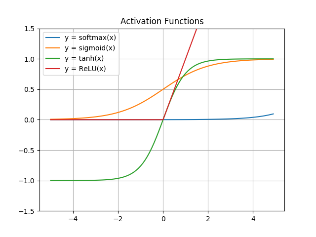
4-2. Comparison by Visualisation

import matplotlib.pyplot as plt

x = np.arange(-5.0, 5.0, 0.1)
plt.title('Activation Functions')

plt.plot(x, softmax(x))
plt.plot(x, sigmoid(x))
plt.plot(x, tanh(x))
plt.plot(x, ReLU(x))

plt.ylim(-1.5, 1.5)
plt.legend(['y = softmax(x)', 'y = sigmoid(x)', 'y = tanh(x)', 'y = ReLU(x)'])
plt.grid()
plt.show()

4-3. Outputting final outcome (eg. Softmax)

Softmax function is worth putting an emphasis on, because for most of the time, Softmax function is used as the activation function as the last step in fully connected layers.

# data that are outputted from perceptrons
class_scores = np.array([6.53633456, 4.97468644, 8.767656678, 16.6543235, 9.23489844,
              14.8763765, 15.3625635, 16.8317633, 5.98765434, 9.4398844])

# result array that has gone through softmax
result = softmax(class_scores)

max_index = np.argmax(result)
max_value = result[max_index]

print('Result from Softmax: ', np.round(result, 5))
print('maximum value is {}, which has index {}'.format(np.round(max_value, 5), max_index))

# <Terminal output>
# Result from Softmax: [2.0000e-05 0.0000e+00 1.4000e-04 3.7883e-01 2.3000e-04 6.4020e-02
#                       1.0410e-01 4.5238e-01 1.0000e-05 2.8000e-04]
# maximum value is 0.45238, which has index 7

Next post will discuss how we can train a network with just perceptrons.