
Boston House Price Prediction
Regression is basically a process which predicts the relationship between x and y based on features. This time we are going to practice Linear Regression with Boston House Price Data that are already embedded in scikit-learn datasets.
Useful functions
-
sklearn.metrics.mean_squared_error: famous evaluation method (MSE)
-
np.sqrt(x): square root of tensor x
-
linear_model.coef_ : get
Regression coefficientof the fitted linear model
import numpy as np
import pandas as pd
import matplotlib.pyplot as plt
import seaborn as sns
import sklearn.datasets as datasets
from sklearn.model_selection import train_test_split
from sklearn.linear_model import LinearRegression
from sklearn.metrics import mean_squared_error
BOSTON_DATA = datasets.load_boston()
Simple EDA
# Load both boston data and target, and convert it as dataframe.
def add_target_to_data(dataset):
    # make the raw dataset cleaner and easier to process -> use dataframe
    df = pd.DataFrame(dataset.data, columns=dataset.feature_names)
    # put the target data (price) to the dataframe we just made.
    print("Before adding target: ", df.shape)
    df['PRICE'] = dataset.target
    print("After adding target: {} \n {}\n".format(df.shape, df.head(2)))
    return df
"""
10 features as default.
Why didn't I put all the 13 features? Because n_row=2 and n_col=5 as default.
It will create 10 graphs for each features.
"""
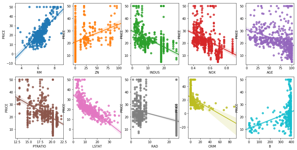
def plotting_graph(df, features, n_row=2, n_col=5):
fig, axes = plt.subplots(n_row, n_col, figsize=(16, 8))
assert len(features) == n_row * n_col
# Draw a regression graph using seaborn's regplot
for i, feature in enumerate(features):
row = int(i / n_col)
col = i % n_col
sns.regplot(x=feature, y='PRICE', data=df, ax=axes[row][col])
plt.show()
def split_dataframe(df):
    label_data = df['PRICE']
    # others without PRICE
    # axis!! --> Whether to drop labels from the index (0 or ‘index’) or columns (1 or ‘columns’).
    input_data = df.drop(['PRICE'], axis=1)

    # split! Set random_state if you want consistently same result
    input_train, input_eval, label_train, label_eval = train_test_split(input_data, label_data, test_size=0.3,
                                                                        random_state=42)

    return input_train, input_eval, label_train, label_eval
boston_df = add_target_to_data(BOSTON_DATA)
features = ['RM', 'ZN', 'INDUS', 'NOX', 'AGE', 'PTRATIO', 'LSTAT', 'RAD', 'CRIM', 'B']
plotting_graph(boston_df, features, n_row=2, n_col=5)
Before adding target:  (506, 13)
After adding target: (506, 14)
       CRIM    ZN  INDUS  CHAS    NOX     RM   AGE     DIS  RAD    TAX  \
0  0.00632  18.0   2.31   0.0  0.538  6.575  65.2  4.0900  1.0  296.0
1  0.02731   0.0   7.07   0.0  0.469  6.421  78.9  4.9671  2.0  242.0

   PTRATIO      B  LSTAT  PRICE
0     15.3  396.9   4.98   24.0
1     17.8  396.9   9.14   21.6
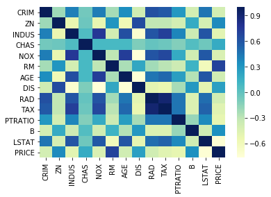
'''
The correlation coefficient ranges from -1 to 1.
If the value is close to 1, it means that there is a strong positive correlation between the two variables.
When it is close to -1, the variables have a strong negative correlation.
'''
correlation_matrix = boston_df.corr().round(2)
Output:
| CRIM | ZN | INDUS | CHAS | NOX | RM | AGE | DIS | RAD | TAX | PTRATIO | B | LSTAT | PRICE | |
|---|---|---|---|---|---|---|---|---|---|---|---|---|---|---|
| CRIM | 1.00 | -0.20 | 0.41 | -0.06 | 0.42 | -0.22 | 0.35 | -0.38 | 0.63 | 0.58 | 0.29 | -0.39 | 0.46 | -0.39 |
| ZN | -0.20 | 1.00 | -0.53 | -0.04 | -0.52 | 0.31 | -0.57 | 0.66 | -0.31 | -0.31 | -0.39 | 0.18 | -0.41 | 0.36 |
| INDUS | 0.41 | -0.53 | 1.00 | 0.06 | 0.76 | -0.39 | 0.64 | -0.71 | 0.60 | 0.72 | 0.38 | -0.36 | 0.60 | -0.48 |
| CHAS | -0.06 | -0.04 | 0.06 | 1.00 | 0.09 | 0.09 | 0.09 | -0.10 | -0.01 | -0.04 | -0.12 | 0.05 | -0.05 | 0.18 |
| NOX | 0.42 | -0.52 | 0.76 | 0.09 | 1.00 | -0.30 | 0.73 | -0.77 | 0.61 | 0.67 | 0.19 | -0.38 | 0.59 | -0.43 |
| RM | -0.22 | 0.31 | -0.39 | 0.09 | -0.30 | 1.00 | -0.24 | 0.21 | -0.21 | -0.29 | -0.36 | 0.13 | -0.61 | 0.70 |
| AGE | 0.35 | -0.57 | 0.64 | 0.09 | 0.73 | -0.24 | 1.00 | -0.75 | 0.46 | 0.51 | 0.26 | -0.27 | 0.60 | -0.38 |
| DIS | -0.38 | 0.66 | -0.71 | -0.10 | -0.77 | 0.21 | -0.75 | 1.00 | -0.49 | -0.53 | -0.23 | 0.29 | -0.50 | 0.25 |
| RAD | 0.63 | -0.31 | 0.60 | -0.01 | 0.61 | -0.21 | 0.46 | -0.49 | 1.00 | 0.91 | 0.46 | -0.44 | 0.49 | -0.38 |
| TAX | 0.58 | -0.31 | 0.72 | -0.04 | 0.67 | -0.29 | 0.51 | -0.53 | 0.91 | 1.00 | 0.46 | -0.44 | 0.54 | -0.47 |
| PTRATIO | 0.29 | -0.39 | 0.38 | -0.12 | 0.19 | -0.36 | 0.26 | -0.23 | 0.46 | 0.46 | 1.00 | -0.18 | 0.37 | -0.51 |
| B | -0.39 | 0.18 | -0.36 | 0.05 | -0.38 | 0.13 | -0.27 | 0.29 | -0.44 | -0.44 | -0.18 | 1.00 | -0.37 | 0.33 |
| LSTAT | 0.46 | -0.41 | 0.60 | -0.05 | 0.59 | -0.61 | 0.60 | -0.50 | 0.49 | 0.54 | 0.37 | -0.37 | 1.00 | -0.74 |
| PRICE | -0.39 | 0.36 | -0.48 | 0.18 | -0.43 | 0.70 | -0.38 | 0.25 | -0.38 | -0.47 | -0.51 | 0.33 | -0.74 | 1.00 |
sns.heatmap(correlation_matrix, cmap="YlGnBu")
plt.show()
Prediction with Linear Regression
X_train, X_test, Y_train, Y_test = split_dataframe(boston_df)

# Load your machine learning model
model = LinearRegression()
# Train!
model.fit(X_train, Y_train)
# make prediction with unseen data!
pred = model.predict(X_test)
expectation = Y_test
# what is mse between the answer and your prediction?
lr_mse = mean_squared_error(expectation, pred)
lr_rmse = np.sqrt(lr_mse)

print('LR_MSE: {0:.3f}, LR_RMSE: {1:.3F}'.format(lr_mse, lr_rmse))
# Regression Coefficient
print('Regression Coefficients:', np.round(model.coef_, 1))
# sort from the biggest
coeff = pd.Series(data=model.coef_, index=X_train.columns).sort_values(ascending=False)
print(coeff)
Output:
LR_MSE: 21.517, LR_RMSE: 4.639
Regression Coefficients: [ -0.1   0.    0.    3.1 -15.4   4.1  -0.   -1.4   0.2  -0.   -0.9   0.
  -0.5]
RM          4.057199
CHAS        3.119835
RAD         0.242727
INDUS       0.049523
ZN          0.035809
B           0.011794
TAX        -0.008702
AGE        -0.010821
CRIM       -0.133470
LSTAT      -0.547113
PTRATIO    -0.910685
DIS        -1.385998
NOX       -15.417061
dtype: float64
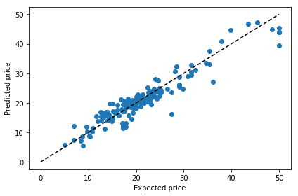
plt.scatter(expectation, pred)
plt.plot([0, 50], [0, 50], '--k')
plt.xlabel('Expected price')
plt.ylabel('Predicted price')
plt.tight_layout()

Prediction with other Regression methods
- Ridge, Lasso and ElasticNet
- Gradient Boosting Regressor
- XG Boost
- SGD Regressor According to sklearn’s official documentation,
“SGDRegressor is well suited for regression problems with a large number of training samples (> 10,000), for other problems we recommend Ridge, Lasso, or ElasticNet.”
from sklearn.linear_model import Ridge, Lasso, ElasticNet, SGDRegressor
from sklearn.ensemble import GradientBoostingRegressor
from xgboost import XGBRegressor
# Try tuning the hyper-parameters
models = {
    "Ridge" : Ridge(),
    "Lasso" : Lasso(),
    "ElasticNet" : ElasticNet(),
    "Gradient Boosting" : GradientBoostingRegressor(),
    "SGD" : SGDRegressor(max_iter=1000, tol=1e-3),
    "XGB" : XGBRegressor(objective ='reg:linear', colsample_bytree = 0.3, learning_rate = 0.1,
                max_depth = 5, alpha = 10, n_estimators = 10)
}

pred_record = {}
for name, model in models.items():
    # Load your machine learning model
    curr_model = model
    # Train!
    curr_model.fit(X_train, Y_train)
    # make prediction with unseen data!
    pred = curr_model.predict(X_test)
    expectation = Y_test
    # what is mse between the answer and your prediction?
    mse = mean_squared_error(expectation, pred)
    rmse = np.sqrt(mse)

    print('{} MSE: {}, {} RMSE: {}'.format(name, mse, name, rmse))

    pred_record.update({name : pred})
Output:
Ridge MSE: 22.044053089861013, Ridge RMSE: 4.695109486461526
Lasso MSE: 25.639502928043992, Lasso RMSE: 5.063546477326341
ElasticNet MSE: 25.40519636428209, ElasticNet RMSE: 5.040356769543411
Gradient Boosting MSE: 7.737869423986623, Gradient Boosting RMSE: 2.781702612427616
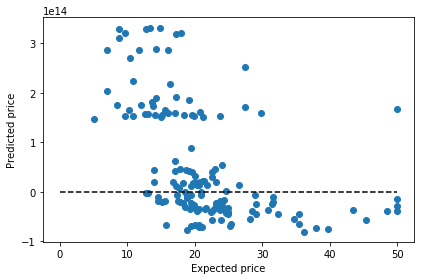
SGD MSE: 1.5570858695910825e+28, SGD RMSE: 124783246855941.47
[20:06:46] WARNING: src/objective/regression_obj.cu:152: reg:linear is now deprecated in favor of reg:squarederror.
XGB MSE: 82.71679422016705, XGB RMSE: 9.094877361469315
prediction = pred_record["SGD"]

plt.scatter(expectation, prediction)
plt.plot([0, 50], [0, 50], '--k')
plt.xlabel('Expected price')
plt.ylabel('Predicted price')
plt.tight_layout()
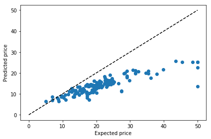
prediction = pred_record["XGB"]

plt.scatter(expectation, prediction)
plt.plot([0, 50], [0, 50], '--k')
plt.xlabel('Expected price')
plt.ylabel('Predicted price')
plt.tight_layout()
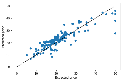
prediction = pred_record["Gradient Boosting"]

plt.scatter(expectation, prediction)
plt.plot([0, 50], [0, 50], '--k')
plt.xlabel('Expected price')
plt.ylabel('Predicted price')
plt.tight_layout()
A Little Taster Session for Neural Network
from tensorflow import keras
from tensorflow.keras.layers import add, Dense, Activation

def neural_net():
    model = keras.Sequential()
    model.add(Dense(512, input_dim=BOSTON_DATA.data.shape[1]))
    model.add(Activation('relu'))
    model.add(Dense(256))
    model.add(Activation('relu'))
    model.add(Dense(128))
    model.add(Activation('relu'))
    model.add(Dense(64))
    model.add(Activation('relu'))
    model.add(Dense(1))
    return model
model = neural_net()
model.summary()
Output:
Model: "sequential_10"
_________________________________________________________________
Layer (type)                 Output Shape              Param #
=================================================================
dense_31 (Dense)             (None, 512)               7168
_________________________________________________________________
activation_24 (Activation)   (None, 512)               0
_________________________________________________________________
dense_32 (Dense)             (None, 256)               131328
_________________________________________________________________
activation_25 (Activation)   (None, 256)               0
_________________________________________________________________
dense_33 (Dense)             (None, 128)               32896
_________________________________________________________________
activation_26 (Activation)   (None, 128)               0
_________________________________________________________________
dense_34 (Dense)             (None, 64)                8256
_________________________________________________________________
activation_27 (Activation)   (None, 64)                0
_________________________________________________________________
dense_35 (Dense)             (None, 1)                 65
=================================================================
Total params: 179,713
Trainable params: 179,713
Non-trainable params: 0
_________________________________________________________________
model.compile(loss='mse', optimizer='adam', metrics=['accuracy'])
history = model.fit(X_train, Y_train, epochs=100)

loss, test_acc = model.evaluate(X_test, Y_test)
print('Test Loss : {:.4f} | Test Accuracy : {}'.format(loss, test_acc))
prediction = model.predict(X_test)

plt.scatter(expectation, prediction)
plt.plot([0, 50], [0, 50], '--k')
plt.xlabel('Expected price')
plt.ylabel('Predicted price')
plt.tight_layout()

Leave a comment