Linear and Polynomial Regressions

Linear Regression from Scratch

Step-by-step guide of Linear Regression

1. Define a function that computes ‘ax+b’
2. Calculate the difference of prediction (y_hat) and y
3. Define how you are going to update ‘a’ and ‘b’, and change their value
4. Iterate above

import numpy as np
import matplotlib.pyplot as plt
import matplotlib as mpl

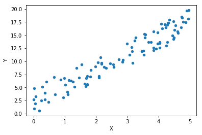
x = 5 * np.random.rand(100, 1)
y = 3 * x + 5 * np.random.rand(100, 1)

# look how our data look like
plt.scatter(x, y, alpha=1, s=20)
plt.xlabel("X")
plt.ylabel("Y")

'''
Step 1
Define a function that computes 'ax+b'
outputs predicted array'''

def prediction(a, b, x):
    # returns 'x*(transposed)a + b'
    equation = np.dot(x, a.T) + b
    return equation

'''Step 2
2. Calculate the difference of prediction and y
'''
learning_rate = 1e-4

def caculate_error(a, b, x, y):
    error = y - prediction(a, b, x)
    return error

'''Step 3
3. Define how you are going to updata 'a' and 'b'
'''
# By how much are you going to update a and b?
def update_ab(a, b, x, error, lr):
    # Update a
    delta_a = -(lr * (2 / len(error)) * (np.dot(x.T, error)))
    # Update b
    delta_b = -(lr * (2 / len(error)) * np.sum(error))

    return delta_a, delta_b

'''Step 4
4. step 2 and step 3 within iteration
'''
# calculate error for given number of times, and update a and b
def gradient_descent(x, y, iteration):
    # initial a and b set to a=0 and b=0
    a = np.zeros((1, 1))
    b = np.zeros((1, 1))

    for i in range(iteration):
        
        #  get errors
        error = caculate_error(a, b, x, y)
        
        # get 'delta'ed a and b
        delta_a, delta_b = update_ab(a, b, x, error, learning_rate)
        # update a and b
        a -= delta_a
        b -= delta_b

    return a, b

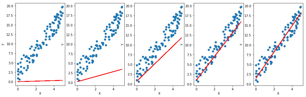
iterations = [10, 100, 500, 1000, 10000]

fig, ax = plt.subplots(1, 5, figsize=(17, 5))

for index, iteration in enumerate(iterations):
    final_a, final_b = gradient_descent(x, y, iteration=iteration)
    print("final a:", final_a, "final b:", final_b)

    # Visualise 5 iteration graphs
    # y_pred = final_a[0][0] * x + final_b
    y_pred = prediction(final_a, final_b, x)
    ax[index].scatter(x, y)
    ax[index].plot(x, y_pred, color='r')
    ax[index].set_xlabel('X')
    ax[index].set_ylabel('Y')

plt.show()

Output:

final a: [[0.07184569]] final b: [[0.0211338]]
final a: [[0.65487756]] final b: [[0.19309695]]
final a: [[2.24708742]] final b: [[0.67068778]]
final a: [[3.03095919]] final b: [[0.9212426]]
final a: [[3.35791156]] final b: [[1.39351818]]

Play around with learning rate and iteration, and try to find the best learning rate!
What if learning rate is very big? What if it’s very small?
What you are doing right now is called Hyper-parameter Tuning / Optimisation!
It is a whole different area, so I will not go very deep into it for now, but I encourage you to Google it.
Let’s get back to this topic after we learn Deep Learning :)

Linear Regression using sklearn

1. Load LR model with
   linear_model = sklearn.linear_model.LinearRegression()

2. Train your model with
   LinearRegression.fit(x, y)

3. Predict y_hat with
   LinearRegression.predict(x)

reference: https://scikit-learn.org/stable/modules/generated/sklearn.linear_model.LinearRegression.html

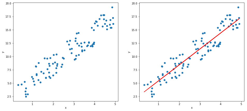
from sklearn.linear_model import LinearRegression

# Load LR model!
model = LinearRegression()

# Train!
model.fit(x, y)

# Predict!
predicted = model.predict(x)

# Visualise
fig, ax = plt.subplots(1, 2, figsize=(16, 7))

ax[0].scatter(x, y)
ax[1].scatter(x, y)
ax[1].plot(x, predicted, color='r')

ax[0].set_xlabel('x')
ax[0].set_ylabel('y')
ax[1].set_xlabel('x')
ax[1].set_ylabel('y')
plt.show()

Multiple Linear Regression

Good mathematical explanation

Another good explanation

import csv
csvReader = csv.reader(open("./data/data.csv"))
# skip the header
next(csvReader)

x = []
y = []

for row in csvReader:
    x_i = [float(row[1]), float(row[2]), float(row[3])]
    x.append(x_i)

    y_i = float(row[4])
    y.append(y_i)

X = np.array(x)
Y = np.array(y)
print(X.shape)
print(Y.shape)
assert len(X)==len(Y)

(200, 3)
(200,)

# Load linear regression model
model = LinearRegression()
# Fit the model!
model.fit(X, Y)
Y_pred = model.predict(X)

print(model.coef_)
print(model.intercept_)
beta_0 = model.coef_[0]   # Facebook
beta_1 = model.coef_[1]   # Instagram
beta_2 = model.coef_[2]   # Twitter
beta_3 = model.intercept_

Output:

[ 0.04576465  0.18853002 -0.00103749]
2.938889369459405

# Inference
# infer an expected sales based on given values
def expected_sales(fb, insta, twitter, beta_0, beta_1, beta_2, beta_3):
    # Multiple Linear Regression Model
    sales = (beta_0 * fb) + (beta_1 * insta) + (beta_2 * twitter) + beta_3
    return sales

# Sales prediction
expectation = expected_sales(100, 200, 0, beta_0, beta_1, beta_2, beta_3)
print("Expected Sales: {}".format(expectation))

# Question: What do you get for (1, 0, 0), (0, 1, 0), (0, 0, 1) and (0, 0, 0)

This is the output: Expected Sales: 45.221357298640044.
Let me ask you one question. What do you get for expected_sales (1, 0, 0), (0, 1, 0), (0, 0, 1) and (0, 0, 0) ?
I’ve already told you the answer!

Polynomial Regression

Let’s do Polynomial Regression using scikit-learn!

What if our training points are non-linear and resemble curvy cosine or cubic function? We need Polynomial Regression, which is often called as Multivariate Regression

PolynomialFeatures(degree): creates Polynomial object
degree: Degree of the polynomial

PolynomialFeatures.fit_transform(x): returns polynomial variables, which are ‘x’ and ‘x to the power of degree’

Check this link out!!
sklearn document

from sklearn.preprocessing import PolynomialFeatures

# Random generation of x and y
x = 3 * np.random.rand(100, 3) + 1
y = (x ** 2) + x + 2 + 5 * np.random.rand(100, 3)

print("x.shape: ", x.shape)

# Create PolynomialFeature object(degree=2, include_bias=False)
poly_feat = PolynomialFeatures(degree=2)

# transform your data (eg: x=[x1, x2] --> poly_x=[1, x1, x2, x1^2, x1x2, x2^2])
poly_x = poly_feat.fit_transform(x)
print("poly_x.shape: ", poly_x.shape)

# Load a model. Which model should you load?
linear_model = LinearRegression()

# fit your model
linear_model.fit(poly_x, y);

Output:

x.shape:  (100, 3)
poly_x.shape:  (100, 10)

Wow!! Now we know that Polynomial Regression is nothing but a variation of Multiple Linear Regression!!!

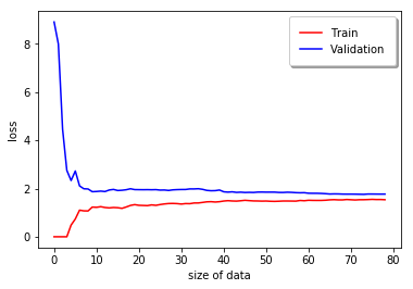
from sklearn.metrics import mean_squared_error as mse
from sklearn.model_selection import train_test_split

def plotting_learning_curves(model, x, y):
    # split your data into train and validation (8:2)
    x_train, x_val, y_train, y_val = train_test_split(x, y, test_size=0.2)
    len_train = len(x_train)

    train_errors = []
    validation_errors = []

    for i in range(1, len_train):
        model.fit(x_train[:i], y_train[:i])
        pred_train = model.predict(x_train[:i])
        pred_val = model.predict(x_val)

        # get mean squared error of train data
        train_error = mse(y_train[:i], pred_train)

        # get mean squared error of validation data
        validation_error = mse(y_val, pred_val)

        train_errors.append(train_error)
        validation_errors.append(validation_error)

    # plotting part
    plt.plot(np.sqrt(train_errors), 'r', label="Train")
    plt.plot(np.sqrt(validation_errors), 'b', label="Validation")

    plt.xlabel("size of data")
    plt.ylabel("loss")

    plt.legend(
        loc='upper right',
        shadow=True,
        fancybox=True,
        borderpad=1  # border padding of the legend box
    )

    plt.show()


plotting_learning_curves(linear_model, x, y)

Other Regressions

Ridge
Lasso
Elastic-Net

1. load Ridge model with
   sklearn.linear_model.Ridge(alpha) alpha: scalar value

2. load Lasso with
   sklearn.linear_model.Lasso(alpha) alpha: scalar value

3. load ElasticNet with
   sklearn.linear_model.ElasticNet(alpha, l1_ratio) alpha: scalar value l1_ratio: ratio for L1 norm

from sklearn.linear_model import Ridge
from sklearn.linear_model import Lasso
from sklearn.linear_model import ElasticNet

# Random generation of x and y
x = 5 * np.random.rand(100, 1)
y = 3 * x + 5 * np.random.rand(100, 1)

# Load Ridge and Train it!
ridge_reg = Ridge(alpha=1.0)
ridge_reg.fit(x, y)

# Load Lasso and Train it!
lasso_reg = Lasso(alpha=0.05)
lasso_reg.fit(x, y)

# Load ElasticNet and Train it!
elastic_net = ElasticNet(alpha=1.0, l1_ratio=0.5)
elastic_net.fit(x, y)

# Predict!
ridge_y_pred = ridge_reg.predict(x)
lasso_y_pred = lasso_reg.predict(x)
elastic_y_pred = elastic_net.predict(x)

# Graph it!
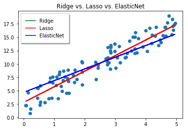
plt.title("Ridge vs. Lasso vs. ElasticNet")
plt.scatter(x, y)

plt.plot(x, ridge_y_pred, color='green', label='Ridge')
plt.plot(x, lasso_y_pred, color='red', label='Lasso')
plt.plot(x, elastic_y_pred, color='blue', label='ElasticNet')

plt.legend(
        loc='upper left',
        shadow=True,
        fancybox=True,
        borderpad=1    # border padding of the legend box
    )

plt.show()